Given the distribution of a discrete random variable, find. Law of distribution of random variables
X; meaning F(5); the probability that the random variable X will take values from the segment . Construct a distribution polygon.
- The distribution function F(x) of a discrete random variable is known X:
Set the law of distribution of a random variable X in the form of a table.
- The law of distribution of a random variable is given X:
| X | –28 | –20 | –12 | –4 | |
| p | 0,22 | 0,44 | 0,17 | 0,1 | 0,07 |
- The probability that the store has quality certificates for the full range of products is 0.7. The commission checked the availability of certificates in four stores in the area. Draw up a distribution law, calculate the mathematical expectation and dispersion of the number of stores in which quality certificates were not found during inspection.
- To determine the average burning time of electric lamps in a batch of 350 identical boxes, one electric lamp from each box was taken for testing. Estimate from below the probability that the average burning duration of the selected electric lamps differs from the average burning duration of the entire batch in absolute value by less than 7 hours, if it is known that the standard deviation of the burning duration of electric lamps in each box is less than 9 hours.
- At a telephone exchange, an incorrect connection occurs with a probability of 0.002. Find the probability that among 500 connections the following will occur:
Find the distribution function of a random variable X. Construct graphs of functions and . Calculate the mathematical expectation, variance, mode and median of a random variable X.
- An automatic machine makes rollers. It is believed that their diameter is a normally distributed random variable with a mean value of 10 mm. What is the standard deviation if, with a probability of 0.99, the diameter is in the range from 9.7 mm to 10.3 mm.
Sample A: 6 9 7 6 4 4
Sample B: 55 72 54 53 64 53 59 48
42 46 50 63 71 56 54 59
54 44 50 43 51 52 60 43
50 70 68 59 53 58 62 49
59 51 52 47 57 71 60 46
55 58 72 47 60 65 63 63
58 56 55 51 64 54 54 63
56 44 73 41 68 54 48 52
52 50 55 49 71 67 58 46
50 51 72 63 64 48 47 55
Option 17.
- Among the 35 parts, 7 are non-standard. Find the probability that two parts taken at random will turn out to be standard.
- Three dice are thrown. Find the probability that the sum of points on the dropped sides is a multiple of 9.
- The word “ADVENTURE” is made up of cards, each with one letter written on it. The cards are shuffled and taken out one at a time without returning. Find the probability that the letters taken out in the order of appearance form the word: a) ADVENTURE; b) PRISONER.
- An urn contains 6 black and 5 white balls. 5 balls are randomly drawn. Find the probability that among them there are:
- 2 white balls;
- less than 2 white balls;
- at least one black ball.
- A in one test is equal to 0.4. Find the probabilities of the following events:
- event A appears 3 times in a series of 7 independent trials;
- event A will appear no less than 220 and no more than 235 times in a series of 400 trials.
- The plant sent 5,000 good-quality products to the base. The probability of damage to each product in transit is 0.002. Find the probability that no more than 3 products will be damaged during the journey.
- The first urn contains 4 white and 9 black balls, and the second urn contains 7 white and 3 black balls. 3 balls are randomly drawn from the first urn, and 4 from the second urn. Find the probability that all the drawn balls are the same color.
- The law of distribution of a random variable is given X:
Calculate its mathematical expectation and variance.
- There are 10 pencils in the box. 4 pencils are drawn at random. Random value X– the number of blue pencils among those selected. Find the law of its distribution, the initial and central moments of the 2nd and 3rd orders.
- The technical control department checks 475 products for defects. The probability that the product is defective is 0.05. Find, with probability 0.95, the boundaries within which the number of defective products among those tested will be contained.
- At a telephone exchange, an incorrect connection occurs with a probability of 0.003. Find the probability that among 1000 connections the following will occur:
- at least 4 incorrect connections;
- more than two incorrect connections.
- The random variable is specified by the distribution density function:
Find the distribution function of a random variable X. Construct graphs of functions and . Calculate the mathematical expectation, variance, mode and median of the random variable X.
- The random variable is specified by the distribution function:
- By sample A solve the following problems:
- create a variation series;
· sample average;
· sample variance;
Mode and median;
Sample A: 0 0 2 2 1 4
- calculate the numerical characteristics of the variation series:
· sample average;
· sample variance;
standard sample deviation;
· mode and median;
Sample B: 166 154 168 169 178 182 169 159
161 150 149 173 173 156 164 169
157 148 169 149 157 171 154 152
164 157 177 155 167 169 175 166
167 150 156 162 170 167 161 158
168 164 170 172 173 157 157 162
156 150 154 163 143 170 170 168
151 174 155 163 166 173 162 182
166 163 170 173 159 149 172 176
Option 18.
- Among 10 lottery tickets, 2 are winning ones. Find the probability that out of five tickets taken at random, one will be a winner.
- Three dice are thrown. Find the probability that the sum of the rolled points is greater than 15.
- The word “PERIMETER” is made up of cards, each of which has one letter written on it. The cards are shuffled and taken out one at a time without returning. Find the probability that the letters taken out form the word: a) PERIMETER; b) METER.
- An urn contains 5 black and 7 white balls. 5 balls are randomly drawn. Find the probability that among them there are:
- 4 white balls;
- less than 2 white balls;
- at least one black ball.
- Probability of an event occurring A in one trial is equal to 0.55. Find the probabilities of the following events:
- event A will appear 3 times in a series of 5 challenges;
- event A will appear no less than 130 and no more than 200 times in a series of 300 trials.
- The probability of a can of canned goods breaking is 0.0005. Find the probability that among 2000 cans, two will have a leak.
- The first urn contains 4 white and 8 black balls, and the second urn contains 7 white and 4 black balls. Two balls are randomly drawn from the first urn and three balls are randomly drawn from the second urn. Find the probability that all the drawn balls are the same color.
- Among the parts arriving for assembly, 0.1% are defective from the first machine, 0.2% from the second, 0.25% from the third, and 0.5% from the fourth. The machine productivity ratios are respectively 4:3:2:1. The part taken at random turned out to be standard. Find the probability that the part was made on the first machine.
- The law of distribution of a random variable is given X:
Calculate its mathematical expectation and variance.
- An electrician has three light bulbs, each of which has a defect with a probability of 0.1. The light bulbs are screwed into the socket and the current is turned on. When the current is turned on, the defective light bulb immediately burns out and is replaced by another. Find the distribution law, mathematical expectation and dispersion of the number of tested light bulbs.
- The probability of hitting a target is 0.3 for each of 900 independent shots. Using Chebyshev's inequality, estimate the probability that the target will be hit at least 240 times and at most 300 times.
- At a telephone exchange, an incorrect connection occurs with a probability of 0.002. Find the probability that among 800 connections the following will occur:
- at least three incorrect connections;
- more than four incorrect connections.
- The random variable is specified by the distribution density function:
Find the distribution function of the random variable X. Draw graphs of the functions and . Calculate the mathematical expectation, variance, mode and median of a random variable X.
- The random variable is specified by the distribution function:
- By sample A solve the following problems:
- create a variation series;
- calculate relative and accumulated frequencies;
- compile an empirical distribution function and plot it;
- calculate the numerical characteristics of the variation series:
· sample average;
· sample variance;
standard sample deviation;
· mode and median;
Sample A: 4 7 6 3 3 4
- Using sample B, solve the following problems:
- create a grouped variation series;
- build a histogram and frequency polygon;
- calculate the numerical characteristics of the variation series:
· sample average;
· sample variance;
standard sample deviation;
· mode and median;
Sample B: 152 161 141 155 171 160 150 157
154 164 138 172 155 152 177 160
168 157 115 128 154 149 150 141
172 154 144 177 151 128 150 147
143 164 156 145 156 170 171 142
148 153 152 170 142 153 162 128
150 146 155 154 163 142 171 138
128 158 140 160 144 150 162 151
163 157 177 127 141 160 160 142
159 147 142 122 155 144 170 177
Option 19.
1. There are 16 women and 5 men working at the site. 3 people were selected at random using their personnel numbers. Find the probability that all selected people will be men.
2. Four coins are tossed. Find the probability that only two coins will have a “coat of arms”.
3. The word “PSYCHOLOGY” is made up of cards, each of which has one letter written on it. The cards are shuffled and taken out one at a time without returning. Find the probability that the letters taken out form a word: a) PSYCHOLOGY; b) STAFF.
4. The urn contains 6 black and 7 white balls. 5 balls are randomly drawn. Find the probability that among them there are:
a. 3 white balls;
b. less than 3 white balls;
c. at least one white ball.
5. Probability of an event occurring A in one trial is equal to 0.5. Find the probabilities of the following events:
a. event A appears 3 times in a series of 5 independent trials;
b. event A will appear at least 30 and no more than 40 times in a series of 50 trials.
6. There are 100 machines of the same power, operating independently of each other in the same mode, in which their drive is turned on for 0.8 working hours. What is the probability that at any given moment in time from 70 to 86 machines will be turned on?
7. The first urn contains 4 white and 7 black balls, and the second urn contains 8 white and 3 black balls. 4 balls are randomly drawn from the first urn, and 1 ball from the second. Find the probability that among the drawn balls there are only 4 black balls.
8. The car sales showroom receives cars of three brands daily in volumes: “Moskvich” – 40%; "Oka" - 20%; "Volga" - 40% of all imported cars. Among Moskvich cars, 0.5% have an anti-theft device, Oka – 0.01%, Volga – 0.1%. Find the probability that the car taken for inspection has an anti-theft device.
9. Numbers and are chosen at random on the segment. Find the probability that these numbers satisfy the inequalities.
10. The law of distribution of a random variable is given X:
| X | ||||
| p | 0,1 | 0,2 | 0,3 | 0,4 |
Find the distribution function of a random variable X; meaning F(2); the probability that the random variable X will take values from the interval . Construct a distribution polygon.
As is known, random variable is called a variable quantity that can take on certain values depending on the case. Random variables are denoted by capital letters of the Latin alphabet (X, Y, Z), and their values are denoted by corresponding lowercase letters (x, y, z). Random variables are divided into discontinuous (discrete) and continuous.
Discrete random variable is a random variable that takes only a finite or infinite (countable) set of values with certain non-zero probabilities.
Distribution law of a discrete random variable is a function that connects the values of a random variable with their corresponding probabilities. The distribution law can be specified in one of the following ways.
1 . The distribution law can be given by the table:
where λ>0, k = 0, 1, 2, … .
V) by using distribution function F(x) , which determines for each value x the probability that the random variable X will take a value less than x, i.e. F(x) = P(X< x).
Properties of the function F(x)
3 . The distribution law can be specified graphically – distribution polygon (polygon) (see problem 3).
Note that to solve some problems it is not necessary to know the distribution law. In some cases, it is enough to know one or several numbers that reflect the most important features of the distribution law. This can be a number that has the meaning of the “average value” of a random variable, or a number showing the average size of the deviation of a random variable from its mean value. Numbers of this kind are called numerical characteristics of a random variable.
Basic numerical characteristics of a discrete random variable :
- Mathematical expectation
(average value) of a discrete random variable M(X)=Σ x i p i.
For binomial distribution M(X)=np, for Poisson distribution M(X)=λ - Dispersion
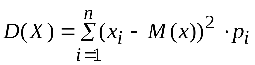
discrete random variable D(X)=M2 or D(X) = M(X 2)− 2. The difference X–M(X) is called the deviation of a random variable from its mathematical expectation.
For binomial distribution D(X)=npq, for Poisson distribution D(X)=λ - Standard deviation (standard deviation) σ(X)=√D(X).
Examples of solving problems on the topic “The law of distribution of a discrete random variable”
Task 1.
1000 lottery tickets were issued: 5 of them will win 500 rubles, 10 will win 100 rubles, 20 will win 50 rubles, 50 will win 10 rubles. Determine the law of probability distribution of the random variable X - winnings per ticket.
Solution. According to the conditions of the problem, the following values of the random variable X are possible: 0, 10, 50, 100 and 500.
The number of tickets without winning is 1000 – (5+10+20+50) = 915, then P(X=0) = 915/1000 = 0.915.
Similarly, we find all other probabilities: P(X=0) = 50/1000=0.05, P(X=50) = 20/1000=0.02, P(X=100) = 10/1000=0.01 , P(X=500) = 5/1000=0.005. Let us present the resulting law in the form of a table:
Let's find the mathematical expectation of the value X: M(X) = 1*1/6 + 2*1/6 + 3*1/6 + 4*1/6 + 5*1/6 + 6*1/6 = (1+ 2+3+4+5+6)/6 = 21/6 = 3.5
Task 3.
The device consists of three independently operating elements. The probability of failure of each element in one experiment is 0.1. Draw up a distribution law for the number of failed elements in one experiment, construct a distribution polygon. Find the distribution function F(x) and plot it. Find the mathematical expectation, variance and standard deviation of a discrete random variable.
Solution. 1. The discrete random variable X = (the number of failed elements in one experiment) has the following possible values: x 1 = 0 (none of the device elements failed), x 2 = 1 (one element failed), x 3 = 2 (two elements failed ) and x 4 =3 (three elements failed).
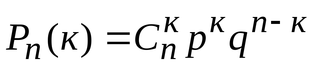
Failures of elements are independent of each other, the probabilities of failure of each element are equal, therefore it is applicable Bernoulli formula
. Considering that, according to the condition, n=3, p=0.1, q=1-p=0.9, we determine the probabilities of the values:
P 3 (0) = C 3 0 p 0 q 3-0 = q 3 = 0.9 3 = 0.729;
P 3 (1) = C 3 1 p 1 q 3-1 = 3*0.1*0.9 2 = 0.243;
P 3 (2) = C 3 2 p 2 q 3-2 = 3*0.1 2 *0.9 = 0.027;
P 3 (3) = C 3 3 p 3 q 3-3 = p 3 =0.1 3 = 0.001;
Check: ∑p i = 0.729+0.243+0.027+0.001=1.
Thus, the desired binomial distribution law of X has the form:
We plot the possible values of x i along the abscissa axis, and the corresponding probabilities p i along the ordinate axis. Let's construct points M 1 (0; 0.729), M 2 (1; 0.243), M 3 (2; 0.027), M 4 (3; 0.001). By connecting these points with straight line segments, we obtain the desired distribution polygon.
3. Let's find the distribution function F(x) = Р(Х
For x ≤ 0 we have F(x) = Р(Х<0) = 0;for 0< x ≤1 имеем F(x) = Р(Х<1) = Р(Х = 0) = 0,729;
for 1< x ≤ 2 F(x) = Р(Х<2) = Р(Х=0) + Р(Х=1) =0,729+ 0,243 = 0,972;
for 2< x ≤ 3 F(x) = Р(Х<3) = Р(Х = 0) + Р(Х = 1) + Р(Х = 2) = 0,972+0,027 = 0,999;
for x > 3 there will be F(x) = 1, because the event is reliable.
 |
Graph of function F(x)
4.
For binomial distribution X:
- mathematical expectation M(X) = np = 3*0.1 = 0.3;
- variance D(X) = npq = 3*0.1*0.9 = 0.27;
- standard deviation σ(X) = √D(X) = √0.27 ≈ 0.52.
LAW OF DISTRIBUTION AND CHARACTERISTICS
RANDOM VARIABLES
Random variables, their classification and methods of description.
A random quantity is a quantity that, as a result of experiment, can take on one or another value, but which one is not known in advance. For a random variable, therefore, you can only specify values, one of which it will definitely take as a result of experiment. In what follows we will call these values possible values of the random variable. Since a random variable quantitatively characterizes the random result of an experiment, it can be considered as a quantitative characteristic of a random event.
Random variables are usually denoted by capital letters of the Latin alphabet, for example, X..Y..Z, and their possible values by corresponding small letters.
There are three types of random variables:
Discrete; Continuous; Mixed.
Discrete is a random variable whose number of possible values forms a countable set. In turn, a set whose elements can be numbered is called countable. The word "discrete" comes from the Latin discretus, meaning "discontinuous, consisting of separate parts".
Example 1. A discrete random variable is the number of defective parts X in a batch of nproducts. Indeed, the possible values of this random variable are a series of integers from 0 to n.
Example 2. A discrete random variable is the number of shots before the first hit on the target. Here, as in Example 1, the possible values can be numbered, although in the limiting case the possible value is an infinitely large number.
Continuous is a random variable whose possible values continuously fill a certain interval of the numerical axis, sometimes called the interval of existence of this random variable. Thus, on any finite interval of existence, the number of possible values of a continuous random variable is infinitely large.
Example 3. A continuous random variable is the monthly electricity consumption of an enterprise.
Example 4. A continuous random variable is the error in measuring height using an altimeter. Let it be known from the operating principle of the altimeter that the error lies in the range from 0 to 2 m. Therefore, the interval of existence of this random variable is the interval from 0 to 2 m.
Law of distribution of random variables.
A random variable is considered completely specified if its possible values are indicated on the numerical axis and the distribution law is established.
Law of distribution of a random variable is a relation that establishes a connection between the possible values of a random variable and the corresponding probabilities.
A random variable is said to be distributed according to a given law, or subject to a given distribution law. A number of probabilities, distribution function, probability density, and characteristic function are used as distribution laws.
The distribution law gives a complete probable description of a random variable. According to the distribution law, one can judge before experiment which possible values of a random variable will appear more often and which less often.
For a discrete random variable, the distribution law can be specified in the form of a table, analytically (in the form of a formula) and graphically.
The simplest form of specifying the distribution law of a discrete random variable is a table (matrix), which lists in ascending order all possible values of the random variable and their corresponding probabilities, i.e.
![]()
Such a table is called a distribution series of a discrete random variable. 1
Events X 1, X 2,..., X n, consisting in the fact that as a result of the test, the random variable X will take the values x 1, x 2,... x n, respectively, are inconsistent and the only possible ones (since the table lists all possible values of a random variable), i.e. form a complete group. Therefore, the sum of their probabilities is equal to 1. Thus, for any discrete random variable
![]()
(This unit is somehow distributed among the values of the random variable, hence the term "distribution").
The distribution series can be depicted graphically if the values of the random variable are plotted along the abscissa axis, and their corresponding probabilities are plotted along the ordinate axis. The connection of the obtained points forms a broken line, called a polygon or polygon of the probability distribution (Fig. 1).

Example The lottery includes: a car worth 5,000 den. units, 4 TVs costing 250 den. units, 5 video recorders worth 200 den. units A total of 1000 tickets are sold for 7 days. units Draw up a distribution law for the net winnings received by a lottery participant who bought one ticket.
Solution. Possible values of the random variable X - the net winnings per ticket - are equal to 0-7 = -7 money. units (if the ticket did not win), 200-7 = 193, 250-7 = 243, 5000-7 = 4993 den. units (if the ticket has the winnings of a VCR, TV or car, respectively). Considering that out of 1000 tickets the number of non-winners is 990, and the indicated winnings are 5, 4 and 1, respectively, and using the classical definition of probability, we obtain.
A distribution series of a discrete random variable is given. Find the missing probability and plot the distribution function. Calculate the mathematical expectation and variance of this quantity.
The random variable X takes only four values: -4, -3, 1 and 2. It takes each of these values with a certain probability. Since the sum of all probabilities must be equal to 1, the missing probability is equal to:
0,3 + ? + 0,1 + 0,4 = 1,
Let's compose the distribution function of the random variable X. It is known that the distribution function , then:

Hence,

Let's plot the function F(x) .

The mathematical expectation of a discrete random variable is equal to the sum of the products of the value of the random variable and the corresponding probability, i.e.
We find the variance of a discrete random variable using the formula:
APPLICATION
Elements of combinatorics Here: - factorial of a number |
||||||||||
Actions on eventsAn event is any fact that may or may not happen as a result of an experience. Merging Events A And IN- this event WITH which consists of an appearance or event A, or events IN, or both events simultaneously. Designation: Crossing Events A And IN- this event WITH, which consists of the simultaneous occurrence of both events. Designation: |
||||||||||
Classic definition of probabilityProbability of event A is the ratio of the number of experiments
|
||||||||||
Probability multiplication formulaProbability of event
If events A and B are independent (the occurrence of one does not affect the occurrence of the other), then the probability of the event is equal to: |
||||||||||
Formula for adding probabilitiesThe probability of an event can be found using the formula: Probability of event A, Probability of event IN,
If events A and B are incompatible (cannot occur simultaneously), then the probability of the event is equal to: |
||||||||||
Total Probability FormulaLet the event A can happen simultaneously with one of the events |
||||||||||
Bernoulli schemeLet there be n independent tests. Probability of occurrence (success) of an event A in each of them is constant and equal p, the probability of failure (i.e. the event not occurring A) q = 1 - p. Then the probability of occurrence k success in n tests can be found using Bernoulli's formula:
Most likely number of successes |
||||||||||
Random variablesdiscrete continuous (for example, the number of girls in a family with 5 children) (for example, the time the kettle works properly) Numerical characteristics of discrete random variablesLet a discrete quantity be given by a distribution series:
, , …, - values of a random variable X; , , …, are the corresponding probability values. Distribution functionDistribution function of a random variable X is a function defined on the entire number line and equal to the probability that X there will be less X: |

 ;
; ;
; , favorable for the occurrence of an event A, to the total number of experiments
  :
:
 can be found using the formula:
 - probability of event A,
 - probability of event IN,
 - probability of event IN provided that the event A has already happened.
 - probability of co-occurrence of events A And IN.
 ,
,
 ,
…,
,
…,
 - let's call them hypotheses. Also known
  - probability of execution i-th hypothesis and
  - probability of occurrence of event A when executing i-th hypothesis. Then the probability of the event A can be found by the formula:
 in the Bernoulli scheme, this is the number of occurrences of some event that has the highest probability. Can be found using the formula:


Questions for the exam
Event. Operations on random events.
The concept of event probability.
Rules for adding and multiplying probabilities. Conditional probabilities.
Total probability formula. Bayes formula.
Bernoulli scheme.
Random variable, its distribution function and distribution series.
Basic properties of the distribution function.
Expected value. Properties of mathematical expectation.
Dispersion. Properties of dispersion.
Probability distribution density of a one-dimensional random variable.
Types of distributions: uniform, exponential, normal, binomial and Poisson distribution.
Local and integral theorems of Moivre-Laplace.
Law and distribution function of a system of two random variables.
Distribution density of a system of two random variables.
Conditional laws of distribution, conditional mathematical expectation.
Dependent and independent random variables. Correlation coefficient.
Sample. Sample processing. Polygon and frequency histogram. Empirical distribution function.
The concept of estimating distribution parameters. Requirements for assessment. Confidence interval. Construction of intervals for estimating mathematical expectation and standard deviation.
Statistical hypotheses. Consent criteria.
In applications of probability theory, the quantitative characteristics of the experiment are of primary importance. A quantity that can be quantitatively determined and which, as a result of an experiment, can take on different values depending on the case is called random variable.
Examples of random variables:
1. The number of times an even number of points appears in ten throws of a die.
2. The number of hits on the target by a shooter who fires a series of shots.
3. The number of fragments of an exploding shell.
In each of the examples given, the random variable can only take on isolated values, that is, values that can be enumerated using a natural series of numbers.
Such a random variable, the possible values of which are individual isolated numbers, which this variable takes with certain probabilities, is called discrete.
The number of possible values of a discrete random variable can be finite or infinite (countable).
Law of distribution A discrete random variable is a list of its possible values and their corresponding probabilities. The distribution law of a discrete random variable can be specified in the form of a table (probability distribution series), analytically and graphically (probability distribution polygon).
When carrying out an experiment, it becomes necessary to evaluate the value being studied “on average.” The role of the average value of a random variable is played by a numerical characteristic called mathematical expectation, which is determined by the formula
Where x 1 , x 2 ,.. , x n– random variable values X, A p 1 ,p 2 , ... , p n– the probabilities of these values (note that p 1 + p 2 +…+ p n = 1).
Example. Shooting is carried out at the target (Fig. 11).

A hit in I gives three points, in II – two points, in III – one point. The number of points scored in one shot by one shooter has a distribution law of the form
To compare the skill of shooters, it is enough to compare the average values of the points scored, i.e. mathematical expectations M(X) And M(Y):
M(X) = 1 0,4 + 2 0,2 + 3 0,4 = 2,0,
M(Y) = 1 0,2 + 2 0,5 + 3 0,3 = 2,1.
The second shooter gives on average a slightly higher number of points, i.e. it will give better results when fired repeatedly.
Let us note the properties of the mathematical expectation:
1. The mathematical expectation of a constant value is equal to the constant itself:
M(C) = C.
2. The mathematical expectation of the sum of random variables is equal to the sum of the mathematical expectations of the terms:
M =(X 1 + X 2 +…+ X n)= M(X 1)+ M(X 2)+…+ M(X n).
3. The mathematical expectation of the product of mutually independent random variables is equal to the product of the mathematical expectations of the factors
M(X 1 X 2 … X n) = M(X 1)M(X 2)… M(X n).
4. The mathematical negation of the binomial distribution is equal to the product of the number of trials and the probability of an event occurring in one trial (task 4.6).
M(X) = pr.
To assess how a random variable “on average” deviates from its mathematical expectation, i.e. In order to characterize the spread of values of a random variable in probability theory, the concept of dispersion is used.
Variance random variable X is called the mathematical expectation of the squared deviation:
D(X) = M[(X - M(X)) 2 ].
Dispersion is a numerical characteristic of the dispersion of a random variable. From the definition it is clear that the smaller the dispersion of a random variable, the more closely its possible values are located around the mathematical expectation, that is, the better the values of the random variable are characterized by its mathematical expectation.
From the definition it follows that the variance can be calculated using the formula
 .
.
It is convenient to calculate the variance using another formula:
D(X) = M(X 2) - (M(X)) 2 .
The dispersion has the following properties:
1. The variance of the constant is zero:
D(C) = 0.
2. The constant factor can be taken out of the dispersion sign by squaring it:
D(CX) = C 2 D(X).
3. The variance of the sum of independent random variables is equal to the sum of the variance of the terms:
D(X 1 + X 2 + X 3 +…+ X n)= D(X 1)+ D(X 2)+…+ D(X n)
4. The variance of the binomial distribution is equal to the product of the number of trials and the probability of the occurrence and non-occurrence of an event in one trial:
D(X) = npq.
In probability theory, a numerical characteristic equal to the square root of the variance of a random variable is often used. This numerical characteristic is called the mean square deviation and is denoted by the symbol
 .
.
It characterizes the approximate size of the deviation of a random variable from its average value and has the same dimension as the random variable.
4.1. The shooter fires three shots at the target. The probability of hitting the target with each shot is 0.3.
Construct a distribution series for the number of hits.
Solution. The number of hits is a discrete random variable X. Each value x n random variable X corresponds to a certain probability P n .
The distribution law of a discrete random variable in this case can be specified near distribution.
In this problem X takes values 0, 1, 2, 3. According to Bernoulli's formula
 ,
,
Let's find the probabilities of possible values of the random variable:
R 3 (0) = (0,7) 3 = 0,343,
R 3 (1)
= 0,3(0,7) 2
= 0,441,
0,3(0,7) 2
= 0,441,
R 3 (2)
= (0,3) 2 0,7
= 0,189,
(0,3) 2 0,7
= 0,189,
R 3 (3) = (0,3) 3 = 0,027.
By arranging the values of the random variable X in increasing order, we obtain the distribution series:
|
X n | ||||
Note that the amount

means the probability that the random variable X will take at least one value from among the possible ones, and this event is reliable, therefore
 .
.
4.2 .There are four balls in the urn with numbers from 1 to 4. Two balls are taken out. Random value X– the sum of the ball numbers. Construct a distribution series of a random variable X.
Solution. Random variable values X are 3, 4, 5, 6, 7. Let's find the corresponding probabilities. Random variable value 3 X can be accepted in the only case when one of the selected balls has the number 1, and the other 2. The number of possible test outcomes is equal to the number of combinations of four (the number of possible pairs of balls) of two.
Using the classical probability formula we get

Likewise,
R(X= 4) =R(X= 6) =R(X= 7) = 1/6.
The sum 5 can appear in two cases: 1 + 4 and 2 + 3, so
 .
.
X has the form:
Find the distribution function F(x) random variable X and plot it. Calculate for X its mathematical expectation and variance.
Solution. The distribution law of a random variable can be specified by the distribution function
F(x) = P(X x).
Distribution function F(x) is a non-decreasing, left-continuous function defined on the entire number line, while
F (- )= 0,F (+ )= 1.
For a discrete random variable, this function is expressed by the formula
 .
.
Therefore in this case

Distribution function graph F(x) is a stepped line (Fig. 12)
|
F(x) | ||||||
Expected valueM(X) is the weighted arithmetic average of the values X 1 , X 2 ,……X n random variable X with scales ρ 1, ρ 2, …… , ρ n and is called the mean value of the random variable X. According to the formula
M(X)= x 1 ρ 1 + x 2 ρ 2 +……+ x n ρ n
M(X) = 3·0.14+5·0.2+7·0.49+11·0.17 = 6.72.
Dispersion characterizes the degree of dispersion of the values of a random variable from its average value and is denoted D(X):
D(X)=M[(HM(X)) 2 ]= M(X 2) –[M(X)] 2 .
For a discrete random variable, the variance has the form

or it can be calculated using the formula
Substituting the numerical data of the problem into the formula, we get:
M(X 2) = 3 2 ∙ 0,14+5 2 ∙ 0,2+7 2 ∙ 0,49+11 2 ∙ 0,17 = 50,84
D(X) = 50,84-6,72 2 = 5,6816.
4.4. Two dice are rolled twice at the same time. Write the binomial law of distribution of a discrete random variable X- the number of occurrences of an even total number of points on two dice.
Solution. Let us introduce a random event
A= (two dice with one throw resulted in a total of even number of points).
Using the classical definition of probability we find
R(A)=
 ,
,
Where n - the number of possible test outcomes is found according to the rule
multiplication:
n = 6∙6 =36,
m - number of people favoring the event A outcomes - equal
m= 3∙6=18.
Thus, the probability of success in one trial is
ρ = P(A)= 1/2.
The problem is solved using a Bernoulli test scheme. One challenge here would be to roll two dice once. Number of such tests n = 2. Random variable X takes values 0, 1, 2 with probabilities
R 2 (0)
= ,R 2 (1)
=
,R 2 (1)
= ∙
∙ ,R 2 (2)
=
,R 2 (2)
=
The required binomial distribution of a random variable X can be represented as a distribution series:
|
X n | |||
|
ρ n |
4.5 . In a batch of six parts there are four standard parts. Three parts were selected at random. Construct a probability distribution of a discrete random variable X– the number of standard parts among those selected and find its mathematical expectation.
Solution. Random variable values X are the numbers 0,1,2,3. It's clear that R(X=0)=0, since there are only two non-standard parts.
R(X=1) = =1/5,
=1/5,
R(X= 2) = = 3/5,
R(X=3) = = 1/5.
Distribution law of a random variable X Let's present it in the form of a distribution series:
|
X n | ||||
|
ρ n |
Expected value
M(X)=1 ∙ 1/5+2 ∙ 3/5+3 ∙ 1/5=2.
4.6 . Prove that the mathematical expectation of a discrete random variable X- number of occurrences of the event A V n independent trials, in each of which the probability of an event occurring is equal to ρ – equal to the product of the number of trials by the probability of the occurrence of an event in one trial, that is, to prove that the mathematical expectation of the binomial distribution
M(X) =n . ρ ,
and dispersion
D(X) =n.p. .
Solution. Random value X can take values 0, 1, 2..., n. Probability R(X= k) is found using Bernoulli’s formula:
R(X=k)= R n(k)=  ρ
To
(1-ρ
) n- To
ρ
To
(1-ρ
) n- To
Distribution series of a random variable X has the form:
|
X n | |||||
|
ρ n |
q n |
|
|
|
 ρq n- 1
 ρq n- 2
 ρ
n
ρ
nWhere q= 1- ρ .
For the mathematical expectation we have the expression:
M(X)= ρq n -
1
+2
ρq n -
1
+2
 ρ
2
q n -
2
+…+.n
ρ
2
q n -
2
+…+.n
 ρ
n
ρ
n
In the case of one test, that is, with n= 1 for random variable X 1 – number of occurrences of the event A- the distribution series has the form:
|
X n | ||
|
ρ n |
M(X 1)= 0∙q + 1 ∙ p = p
D(X 1) = p – p 2 = p(1- p) = pq.
If X k – number of occurrences of the event A in which test, then R(X To)= ρ And
X=X 1 +X 2 +….+X n .
From here we get
M(X)=M(X 1 )+M(X 2)+ … +M(X n)= nρ,
D(X)=D(X 1)+D(X 2)+ ... +D(X n)=npq.
4.7. The quality control department checks products for standardness. The probability that the product is standard is 0.9. Each batch contains 5 products. Find the mathematical expectation of a discrete random variable X- the number of batches, each of which will contain 4 standard products - if 50 batches are subject to inspection.
Solution. The probability that there will be 4 standard products in each randomly selected batch is constant; let's denote it by ρ .Then the mathematical expectation of the random variable X equals M(X)= 50∙ρ.
Let's find the probability ρ according to Bernoulli's formula:
ρ=P 5 (4)= = 0,94∙0,1=0,32.
M(X)= 50∙0,32=16.
4.8 . Three dice are thrown. Find the mathematical expectation of the sum of the dropped points.
Solution. You can find the distribution of a random variable X- the sum of the dropped points and then its mathematical expectation. However, this path is too cumbersome. It is easier to use another technique, representing a random variable X, the mathematical expectation of which needs to be calculated, in the form of a sum of several simpler random variables, the mathematical expectation of which is easier to calculate. If the random variable X i- this is the number of points dropped on i– th bones ( i= 1, 2, 3), then the sum of points X will be expressed in the form
X = X 1 + X 2 + X 3 .
To calculate the mathematical expectation of the original random variable, all that remains is to use the property of mathematical expectation
M(X 1 + X 2 + X 3 )= M(X 1 )+ M(X 2)+ M(X 3 ).
It's obvious that
R(X i = K)= 1/6, TO= 1, 2, 3, 4, 5, 6, i= 1, 2, 3.
Therefore, the mathematical expectation of the random variable X i looks like
M(X i) = 1/6∙1 + 1/6∙2 +1/6∙3 + 1/6∙4 + 1/6∙5 + 1/6∙6 = 7/2,
M(X) = 3∙7/2 = 10,5.
4.9. Determine the mathematical expectation of the number of devices that failed during testing if:
a) the probability of failure for all devices is the same R, and the number of devices under test is equal to n;
b) probability of failure for i – of the device is equal to p i , i= 1, 2, … , n.
Solution. Let the random variable X is the number of failed devices, then
X = X 1 + X 2 + … + X n ,
X i
=

It's clear that
R(X i = 1)= R i , R(X i = 0)= 1– R i ,i= 1, 2, … ,n.
M(X i)= 1∙R i + 0∙(1-R i)=P i ,
M(X)=M(X 1)+M(X 2)+ … +M(X n)=P 1 +P 2 + … + P n .
In case “a” the probability of device failure is the same, that is
R i =p,i= 1, 2, … ,n.
M(X)= n.p..
This answer could be obtained immediately if we notice that the random variable X has a binomial distribution with parameters ( n, p).
4.10. Two dice are thrown simultaneously twice. Write the binomial law of distribution of a discrete random variable X - the number of rolls of an even number of points on two dice.
Solution. Let
A=(rolling an even number on the first dice),
B =(rolling an even number on the second dice).
Getting an even number on both dice in one throw is expressed by the product AB. Then
R
(AB)
= R(A)∙R(IN)
=
 .
.
The result of the second throw of two dice does not depend on the first, so Bernoulli's formula applies when
n = 2,p = 1/4, q = 1– p = 3/4.
Random value X can take values 0, 1, 2 , the probability of which can be found using Bernoulli’s formula:
R(X= 0)= P 2 (0) = q 2 = 9/16,
R(X= 1)= P 2
(1)= C  ,R∙q
=
6/16,
,R∙q
=
6/16,
R(X= 2)= P 2
(2)= C  ,
R 2
=
1/16.
,
R 2
=
1/16.
Distribution series of a random variable X:
4.11. The device consists of a large number of independently operating elements with the same very small probability of failure of each element over time t. Find the average number of refusals over time t elements, if the probability that at least one element will fail during this time is 0.98.
Solution. Number of people who refused over time t elements – random variable X, which is distributed according to Poisson's law, since the number of elements is large, the elements work independently and the probability of failure of each element is small. Average number of occurrences of an event in n tests equals
M(X) = n.p..
Since the probability of failure TO elements from n expressed by the formula
R n
(TO)
 ,
,
where = n.p., then the probability that not a single element will fail during the time t we get at K = 0:
R n (0)= e - .
Therefore, the probability of the opposite event is in time t at least one element fails – equal to 1 - e - . According to the conditions of the problem, this probability is 0.98. From Eq.
1 - e - = 0,98,
e - = 1 – 0,98 = 0,02,
from here = -ln 0,02 4.
So, in time t operation of the device, on average 4 elements will fail.
4.12 . The dice are rolled until a “two” comes up. Find the average number of throws.
Solution. Let's introduce a random variable X– the number of tests that must be performed until the event of interest to us occurs. The probability that X= 1 is equal to the probability that during one throw of the dice a “two” will appear, i.e.
R(X= 1) = 1/6.
Event X= 2 means that on the first test the “two” did not come up, but on the second it did. Probability of event X= 2 is found by the rule of multiplying the probabilities of independent events:
R(X= 2) = (5/6)∙(1/6)
Likewise,
R(X= 3) = (5/6) 2 ∙1/6, R(X= 4) = (5/6) 2 ∙1/6
etc. We obtain a series of probability distributions:
|
(5/6) To ∙1/6 |
The average number of throws (trials) is the mathematical expectation
M(X) = 1∙1/6 + 2∙5/6∙1/6 + 3∙(5/6) 2 ∙1/6 + … + TO (5/6) TO -1 ∙1/6 + … =
1/6∙(1+2∙5/6 +3∙(5/6) 2 + … + TO (5/6) TO -1 + …)
Let's find the sum of the series:
 TOg
TO -1
= (
TOg
TO -1
= ( g TO)
g
g TO)
g
 .
.
Hence,
M(X) = (1/6) (1/ (1 – 5/6) 2 = 6.
Thus, you need to make an average of 6 throws of the dice until a “two” comes up.
4.13. Independent tests are carried out with the same probability of occurrence of the event A in every test. Find the probability of an event occurring A, if the variance of the number of occurrences of an event in three independent trials is 0.63 .
Solution. The number of occurrences of an event in three trials is a random variable X, distributed according to the binomial law. The variance of the number of occurrences of an event in independent trials (with the same probability of occurrence of the event in each trial) is equal to the product of the number of trials by the probabilities of the occurrence and non-occurrence of the event (problem 4.6)
D(X) = npq.
By condition n = 3, D(X) = 0.63, so you can R find from equation
0,63 = 3∙R(1-R),
which has two solutions R 1 = 0.7 and R 2 = 0,3.


